
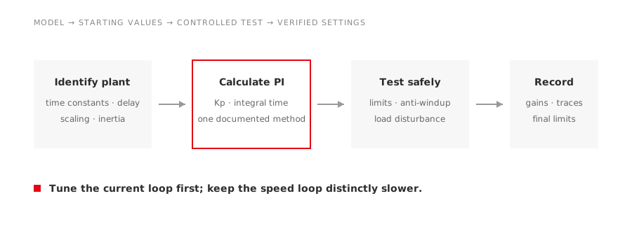
PI tuning becomes difficult when it is treated as a search for two universal numbers. The gains belong to a particular plant model, sampling time, feedback scale and mechanical load. A commissioning method should therefore explain where the first values come from and how the machine proves whether they are acceptable.
Modulus-optimum tuning is one established engineering starting point. It can shape a loop with a dominant plant time constant and smaller delays into a predictable response. It does not replace identification, limit handling or on-machine testing.
What the two terms do
For an error (e), a PI controller produces an output from a proportional term and an accumulated integral term. Proportional action reacts immediately to present error. Integral action keeps adding correction while an error remains, which allows the loop to remove steady-state offset.
Increasing proportional gain usually makes the response faster, but it also amplifies measurement noise and can excite delay or resonance. Stronger integral action removes offset faster, but can increase overshoot and create a slow oscillation if the plant cannot follow the accumulated command.
The right gains are therefore a compromise among response speed, damping, noise, disturbance rejection and actuator limits.
Start with the plant, not the keypad
Before calculating gains, define the loop being tuned. For a current loop, the plant includes the inverter delay, motor inductance and resistance, measurement filters and digital sampling. For a speed loop, it includes the already commissioned current loop, torque constant, combined inertia, friction, load torque and speed feedback.
Record parameters in consistent units. Confirm that current and speed feedback are scaled correctly. A gain calculated in amperes and radians per second will behave incorrectly if the controller internally uses percent current and revolutions per minute.
If reliable parameters are unavailable, use the drive’s approved identification routine or a controlled commissioning test. Do not infer inertia from motor power alone. A flywheel, long coupling, pump column or gearbox can dominate the mechanical model.
Where modulus optimum fits
The modulus-optimum method is useful when the plant can be represented by one main time constant plus smaller delays. The controller zero is chosen to compensate the dominant lag, and the loop gain is selected to obtain a well-damped closed-loop response over the useful bandwidth.
Different textbooks and drive suppliers normalize the equations differently. A formula is only usable when its block diagram, units and definition of total small time constant match the implementation. Copying a result such as “gain equals a constant divided by time” without those definitions is a common commissioning error.
Use the method this way:
- identify the relevant plant transfer function;
- combine the delays that the chosen approximation permits;
- calculate the proportional and integral terms using one documented convention;
- convert them into the drive’s parameter format;
- simulate or test at reduced risk;
- adjust against measured current, speed and saturation behavior.
The method provides a defensible first setting. The commissioning record provides the evidence that it works on the machine.
Tune the current loop first
In a cascaded drive, the inner current loop delivers torque quickly. The outer speed loop asks for the current needed to correct speed. If the current loop is slow, unstable or incorrectly scaled, no speed-loop tuning method can repair it.
Verify current response with the machine secured and within the supplier’s commissioning procedure. Check both positive and negative commands where the application permits. Watch phase current, DC-bus voltage, current limit and any decoupling terms used by vector control.
The current loop should respond cleanly without sustained oscillation or excessive switching noise. Protection limits must remain active during every test.
Keep the speed loop slower
Once the torque-producing current follows its command predictably, tune the speed loop at a lower bandwidth. This separation lets the speed controller treat the current-controlled motor as a faster subsystem.
A speed step is not the only test. Apply a realistic load disturbance and observe:
- peak current and time spent at the current limit;
- speed dip and recovery time;
- overshoot after the load is removed;
- oscillation near mechanical resonance;
- behavior through backlash, stiction or pump torque pulsation;
- temperature and noise during repeated cycles.
For a pumpjack or reciprocating load, a smooth average-speed trace can hide large cyclic torque commands. Trends should include current and torque-producing current, not speed alone.
Deal with limits explicitly
Every drive has voltage, current and torque limits. During acceleration or a large disturbance, the PI output may demand more than the inverter can supply. If the integrator continues accumulating error, the controller “winds up.” When the limit clears, the stored integral term drives overshoot and delays recovery.
Use the manufacturer’s anti-windup function and verify its behavior. Also check acceleration ramps, torque limits and field-weakening transitions. These features interact with the controller and can make a sound set of gains appear poor when the real issue is persistent saturation.
Signs that the model is wrong
Repeated gain reduction is not always the answer. If tuning works unloaded but fails when coupled, revisit the inertia and load model. If oscillation appears only at one speed, investigate structural resonance, coupling stiffness or encoder quality. If the current loop becomes noisy as the motor heats, confirm parameter adaptation and resistance estimation.
Our overview of nested speed and current loops explains why these symptoms appear in different layers. The guide to matching a VFD to a motor covers the hardware checks that tuning cannot fix.
Commissioning evidence to keep
Save the identified parameters, controller convention, final gains, sampling settings, filters, limits and test traces. Include a baseline start, stop, speed change and load disturbance. This record makes later troubleshooting far faster than a screenshot of two gain values.
Good PI tuning is repeatable engineering: model the loop, calculate a starting point, test within limits and document the result. The machine, rather than the reputation of a tuning rule, has the final word.